Amortized Cost Explained and Illustrated for FinOps
This article demystifies amortized cost in the context of FinOps (cloud cost management), explaining and illustrating how cost and usage data reporting can reflect reality and support good decisions.


If you, or someone around you, struggles to understand amortized cost in the context of FinOps (cloud cost management), read or share this article with them. It is often the case with engineers who have not yet been exposed to financials that much, but also finance and controlling folks, who already have an understanding of amortization, but a little bit different due to their distinct context.
Amortization in FinOps and Accounting
The term amortize is borrowed from accounting by cloud cost management. It means to spread a cost over time. The concept of spreading is analogous in both accounting and FinOps, but the "what" and the "why" slightly differ. FinOps has a more specific use case for it.
In accounting, you spread an asset's cost over its useful life. You do this to avoid distorting the financial statements for business decision-makers and to reflect reality by matching the cost to the benefit of the asset (matching principle).
If they did not amortize the cost, they would have a large cost in the first year and nothing in the next two. This would impact the profit (or loss) that they report. In the first year, the large cost would lead to lower profit (or larger loss), and in the next two, a higher profit (or smaller loss), distorting the picture of the business's performance despite operating similarly each year.
In FinOps, you spread a commitment's fee(s) over the commitment's term in the context of Commitment Discounts. You do this to avoid distorting cloud cost reporting for business, product, and engineering folks, who need a consumption and time-proportionate view of costs to avoid drawing the wrong conclusions.
If the provider did not amortize the commitment cost, it would show up as a large spike on the first day of each month, distorting the realistic picture. Cost report users could misinterpret this as an indication that more resources were used on that single day, and fewer on the remaining days of the month, even if resource utilization was actually constant. If they looked at the unit cost, it would also show a distorted picture, much higher than reality for the first day and somewhat lower for the other days.
Understanding Commitment Discounts
For understanding amortization in FinOps, understanding Commitment Discounts in the cloud is essential. If you already know this, skip ahead. Otherwise, read it diligently.
Cloud providers offer their services in multiple ways for purchase. The base scenario is that you buy services at the list prices, i.e., the prices appearing in the public price list without any discount. List prices are also called On-Demand (OD) or Pay-As-You-Go (PAYG) prices by the providers.
If you want to buy at a lower price, cloud providers offer Commitment Discounts. These are similar to traditional volume discounts. The more you buy, the lower the unit price (or rate) gets. However, in the cloud, volume or quantity is measured in different units. Either in terms of usage (of resources) or spend (of money):
- When you commit to usage (e.g., committed use or resource reservation), it is called a Resource-based commitment, and you are saying, "I am going to use the agreed resources for the agreed time".
- When you commit to spend, it is called a Spend-based commitment, and you are saying, "I am going to spend the agreed amount of money for the agreed time".
Commitments carry a financial obligation in the form of a commitment fee. Practically, you are purchasing discount contracts. Think of it this way:
You are paying a commitment fee to have guaranteed access to the usage of cloud resources at a discounted rate.
Therefore, commitment fees are not replacing usage charges in your billing. Technically, they appear as separate billing line items in your cost and usage data. At the same time, to reflect your commitment discount (and any upfront payments), usage is either charged at a lower rate (which can even be zero if the commitment is paid all upfront), or offset with negation or credits.
TERM – The longer term you commit, the more discount you get, because you guarantee a longer-term revenue and cash flow for the provider. Typical commitment terms are one, three and sometimes five years.SPECIFICITY – The more specific resources (type, location) you commit to use, the more discount you get, because you decrease the provider's risk regarding its data center and technology infrastructure utilization, by being specific about the service/resource types, and/or the geographical location you will use (reserve).UPFRONT PAYMENT – The more upfront payment you make, the more discount you get, because money received upfront is immediate and secured, and worth more for the provider than future cashflows (which you generally discount to get their Net Present Value and they are less certain). Not all providers offer upfront payments.FinOps Amortization Illustrated
(Example + Visuals)
Let's say that you are running ten virtual machines in the cloud continuously 24/7. The list price for running a single machine is $1 per hour. Therefore, your cost of running these machines on an on-demand/pay-as-you-go consumption model is:
- Daily $240 (10 × $1 × 24 hrs)
- Monthly $7,300 (10 × $1 × 730 hrs) --> why 730? 👉 check here
- Annually $87,600 (10 × $1 × 730 hrs × 12 months)
You also expect to use these ten machines continually for the following year, so it makes sense for you to take advantage of the provider's offering of a 25% discount in exchange for a one-year commitment. This will reduce your annual cost to $65,700 (75% of $87,600), resulting in a savings of $21,900.
Correspondingly, the provider will charge you a total of $65,700 for the commitment. This amount will be due regardless of whether you actually use the virtual machines or not. So, this is your risk.
Assuming you do not make an upfront payment for the commitment, the provider charges a recurring fee, spread across 12 monthly billing periods (proportional to the number of days in each month). In turn, the provider charges this fee in your monthly billing on the first day of the billing period and then accounts for the actual usage of the virtual machines throughout the month.
Plotting this actual cost (not amortized) on a 30-day chart looks like this.
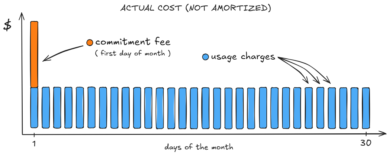
You will immediately realize the challenges with this chart when you want to use it to assess consumption trends. There appears to be a big spike on the first day of the month, suggesting that consumption was higher that day, which is not the case in reality, as a constant consumption is assumed in the example.
If you bring in consumption quantities and calculate the unit cost (per hour of compute), it will also show a much higher unit cost for the first day and a lower one for the other days. This can also lead to misunderstandings.
To fix this issue, the provider will amortize the fee, spreading it proportionally across sub-periods (days, hours, seconds) of the commitment term. I mention multiple time granularities for two reasons. One is that you can choose to report at different granularities, and the other is that different billing line items might use different granularities. For example, compute usage is usually billed on a per-second basis, but discounts are often applied on a per-hour basis.
Let's plot and see how the amortized cost looks on the 30-day chart.
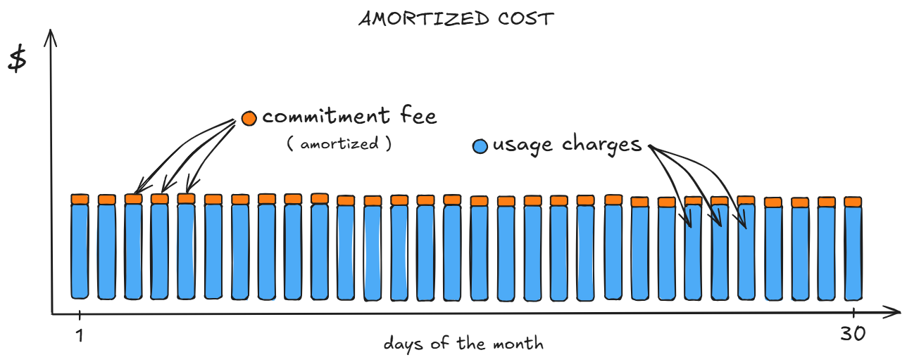
Now it is easy to see how amortized cost provides a more realistic view of consumption and spending trends, proportionate to usage amounts and time sub-periods. At the same time, I must admit that it is also a simplified and generalized representation of how the billing line items in your cost and usage data actually work.
There are three main reasons for this: (1) there are different types of commitment instruments (e.g., reservations, savings plans, committed use discounts), (2) different providers apply different mechanisms to account for discounted usage (rate adjustment, negation, credits), and (3) we did not bake in the concept of upfront payments. I am thinking of addressing these in a separate writing, if you would find that useful, prod me on social.
Terms You Should Also Know About
To complement this explanation of amortization, I have included two related concepts that you may encounter, and which will help you take a broader perspective.
Effective Cost
Effective Cost, in the context of the FOCUS specification, is arguably the most useful column and definition for FinOps practitioners. It incorporates all factors (discounts, commitment fees, amortization, etc.) necessary to provide a realistic view of spending trends over time and perform great FinOps analyses.
Depreciation
In the accounting context, amortization (spreading an asset's cost over its useful life) is applied to intangible assets (the 'untouchables') such as software, copyrights, patents, and trademarks. However, a similar concept also exists for tangible assets (the 'touchables'), such as buildings, vehicles, machines, and equipment. It is called depreciation, and compared to amortization, the key differences are that (1) there is typically a salvage value at the end of a tangible asset's useful life, and (2) the depreciation can follow different methods, e.g., accelerated, and not only an equal, straight-line spread.
You reached the end, great job! I hope you learned something and enjoyed it.
That's my pleasure!